what is the condition for the firm to realize profit
Chapter viii. Perfect Competition
8.two How Perfectly Competitive Firms Make Output Decisions
Learning Objectives
By the end of this department, you will be able to:
- Calculate profits past comparison full revenue and total cost
- Identify profits and losses with the boilerplate cost curve
- Explain the shutdown betoken
- Determine the price at which a house should continue producing in the short run
A perfectly competitive house has merely i major decision to make—namely, what quantity to produce. To sympathise why this is so, consider a different manner of writing out the basic definition of turn a profit:
[latex]\brainstorm{assortment}{r @{{}={}} l}Turn a profit & Total\;revenue\;-\;Total\;cost \\[1em] & (Toll)(Quantity\;produced)\;-\;(Average\;toll)(Quantity\;produced) \end{array}[/latex]
Since a perfectly competitive firm must accept the price for its output as determined by the product's market place demand and supply, it cannot cull the price it charges. This is already determined in the profit equation, and so the perfectly competitive firm can sell any number of units at exactly the same cost. It implies that the firm faces a perfectly elastic demand bend for its product: buyers are willing to buy any number of units of output from the firm at the market price. When the perfectly competitive firm chooses what quantity to produce, then this quantity—along with the prices prevailing in the market place for output and inputs—volition determine the firm'south total acquirement, total costs, and ultimately, level of profits.
Determining the Highest Profit by Comparing Full Revenue and Total Cost
A perfectly competitive firm tin can sell as large a quantity as information technology wishes, as long equally it accepts the prevailing market price. Total revenue is going to increase every bit the firm sells more than, depending on the toll of the product and the number of units sold. If you increase the number of units sold at a given price, then total revenue will increment. If the price of the product increases for every unit of measurement sold, then total revenue also increases. As an example of how a perfectly competitive firm decides what quantity to produce, consider the instance of a pocket-sized farmer who produces raspberries and sells them frozen for $4 per pack. Sales of one pack of raspberries volition bring in $4, two packs will be $eight, three packs volition be $12, and so on. If, for example, the price of frozen raspberries doubles to $viii per pack, then sales of 1 pack of raspberries will be $8, 2 packs will be $16, three packs will be $24, and so on.
Total acquirement and full costs for the raspberry farm, broken downward into fixed and variable costs, are shown in Table i and also appear in Figure 1. The horizontal centrality shows the quantity of frozen raspberries produced in packs; the vertical axis shows both total revenue and total costs, measured in dollars. The total cost curve intersects with the vertical centrality at a value that shows the level of fixed costs, and then slopes upwards. All these cost curves follow the same characteristics as the curves covered in the Cost and Industry Structure affiliate.
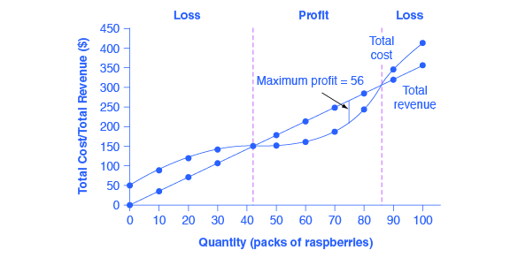
| Quantity (Q) | Total Cost (TC) | Fixed Cost (FC) | Variable Cost (VC) | Total Revenue (TR) | Profit |
|---|---|---|---|---|---|
| 0 | $62 | $62 | – | $0 | −$62 |
| ten | $xc | $62 | $28 | $40 | −$50 |
| 20 | $110 | $62 | $48 | $80 | −$30 |
| thirty | $126 | $62 | $64 | $120 | −$6 |
| twoscore | $144 | $62 | $82 | $160 | $16 |
| 50 | $166 | $62 | $104 | $200 | $34 |
| sixty | $192 | $62 | $130 | $240 | $48 |
| 70 | $224 | $62 | $162 | $280 | $56 |
| 80 | $264 | $62 | $202 | $320 | $56 |
| 90 | $324 | $62 | $262 | $360 | $36 |
| 100 | $404 | $62 | $342 | $400 | −$4 |
| Table 1. Full Price and Full Revenue at the Raspberry Farm | |||||
Based on its total revenue and full cost curves, a perfectly competitive firm like the raspberry subcontract tin calculate the quantity of output that will provide the highest level of profit. At any given quantity, total acquirement minus total cost will equal profit. One style to determine the most profitable quantity to produce is to see at what quantity total revenue exceeds full price by the largest corporeality. On Figure i, the vertical gap between total revenue and total cost represents either turn a profit (if total revenues are greater that total costs at a certain quantity) or losses (if total costs are greater that total revenues at a certain quantity). In this example, total costs will exceed total revenues at output levels from 0 to twoscore, and so over this range of output, the firm will be making losses. At output levels from 50 to 80, total revenues exceed full costs, so the firm is earning profits. But then at an output of 90 or 100, full costs once more exceed total revenues and the firm is making losses. Full profits appear in the final column of Table ane. The highest total profits in the table, as in the figure that is based on the table values, occur at an output of lxx–fourscore, when profits volition be $56.
A higher price would mean that full revenue would be higher for every quantity sold. A lower toll would hateful that total acquirement would exist lower for every quantity sold. What happens if the price drops depression enough and then that the total revenue line is completely below the total price curve; that is, at every level of output, full costs are college than full revenues? In this instance, the best the house tin do is to suffer losses. Just a profit-maximizing firm volition adopt the quantity of output where total revenues come closest to full costs and thus where the losses are smallest.
(Later we volition run across that sometimes it volition make sense for the business firm to shutdown, rather than stay in performance producing output.)
Comparing Marginal Revenue and Marginal Costs
Firms often do not have the necessary data they need to draw a complete total toll bend for all levels of production. They cannot be sure of what total costs would look like if they, say, doubled production or cut production in half, because they accept not tried information technology. Instead, firms experiment. They produce a slightly greater or lower quantity and observe how profits are affected. In economical terms, this practical approach to maximizing profits means looking at how changes in production affect marginal revenue and marginal cost.
Figure two presents the marginal revenue and marginal cost curves based on the full acquirement and full cost in Table ane. The marginal revenue curve shows the additional acquirement gained from selling one more unit. As mentioned before, a firm in perfect competition faces a perfectly elastic need bend for its product—that is, the firm'due south demand bend is a horizontal line drawn at the market place price level. This also means that the firm's marginal acquirement curve is the same equally the firm's need curve: Every time a consumer demands one more unit, the firm sells one more unit and revenue goes upward by exactly the aforementioned amount equal to the market price. In this case, every time a pack of frozen raspberries is sold, the house'due south revenue increases by $4. Tabular array ii shows an example of this. This condition only holds for cost taking firms in perfect contest where:
[latex]marginal\;revenue = cost[/latex]
The formula for marginal revenue is:
[latex]marginal\;revenue = \frac {change\;in\;total\;revenue}{alter\;in\;quantity}[/latex]
| Price | Quantity | Full Revenue | Marginal Revenue |
|---|---|---|---|
| $4 | 1 | $4 | – |
| $4 | 2 | $8 | $4 |
| $4 | iii | $12 | $four |
| $four | 4 | $16 | $four |
| Table 2. Marginal Acquirement | |||
Observe that marginal revenue does not change as the firm produces more output. That is considering the price is adamant by supply and need and does not change as the farmer produces more (keeping in mind that, due to the relative pocket-sized size of each firm, increasing their supply has no impact on the total market supply where price is determined).
Since a perfectly competitive house is a toll taker, it can sell whatever quantity it wishes at the market-determined toll. Marginal cost, the cost per additional unit sold, is calculated by dividing the change in total price by the change in quantity. The formula for marginal price is:
[latex]marginal\;toll = \frac {change\;in\;total\;cost}{change\;in\;quantity}[/latex]
Ordinarily, marginal cost changes as the firm produces a greater quantity.
In the raspberry farm example, shown in Effigy ii, Figure three and Table 3, marginal cost at first declines as production increases from 10 to 20 to 30 packs of raspberries—which represents the surface area of increasing marginal returns that is not uncommon at depression levels of production. But then marginal costs start to increase, displaying the typical pattern of diminishing marginal returns. If the firm is producing at a quantity where MR > MC, like xl or l packs of raspberries, then it can increase profit by increasing output because the marginal revenue is exceeding the marginal cost. If the business firm is producing at a quantity where MC > MR, like 90 or 100 packs, then it tin can increase profit by reducing output because the reductions in marginal toll will exceed the reductions in marginal revenue. The firm's profit-maximizing choice of output will occur where MR = MC (or at a choice close to that bespeak). You will observe that what occurs on the product side is exemplified on the cost side. This is referred to as duality.
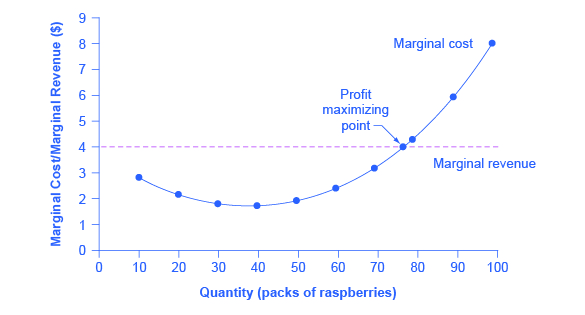
| Quantity | Full Cost | Fixed Cost | Variable Cost | Marginal Price | Full Revenue | Marginal Revenue |
|---|---|---|---|---|---|---|
| 0 | $62 | $62 | – | – | – | – |
| 10 | $90 | $62 | $28 | $2.80 | $xl | $4.00 |
| 20 | $110 | $62 | $48 | $2.00 | $fourscore | $4.00 |
| thirty | $126 | $62 | $64 | $1.60 | $120 | $4.00 |
| 40 | $144 | $62 | $82 | $1.eighty | $160 | $4.00 |
| fifty | $166 | $62 | $104 | $2.20 | $200 | $four.00 |
| 60 | $192 | $62 | $130 | $ii.sixty | $240 | $4.00 |
| 70 | $224 | $62 | $162 | $3.twenty | $280 | $4.00 |
| 80 | $264 | $62 | $202 | $4.00 | $320 | $4.00 |
| ninety | $324 | $62 | $262 | $6.00 | $360 | $four.00 |
| 100 | $404 | $62 | $342 | $8.00 | $400 | $4.00 |
| Tabular array 3. Marginal Revenues and Marginal Costs at the Raspberry Subcontract | ||||||
In this example, the marginal acquirement and marginal toll curves cantankerous at a toll of $four and a quantity of 80 produced. If the farmer started out producing at a level of lx, then experimented with increasing production to 70, marginal revenues from the increase in production would exceed marginal costs—and and so profits would ascension. The farmer has an incentive to continue producing. From a level of 70 to 80, marginal cost and marginal revenue are equal so turn a profit doesn't modify. If the farmer then experimented further with increasing production from 80 to 90, he would find that marginal costs from the increase in production are greater than marginal revenues, so profits would pass up.
The turn a profit-maximizing pick for a perfectly competitive firm volition occur where marginal revenue is equal to marginal cost—that is, where MR = MC. A profit-seeking firm should keep expanding production equally long equally MR > MC. But at the level of output where MR = MC, the firm should recognize that it has achieved the highest possible level of economical profits. (In the example above, the turn a profit maximizing output level is between 70 and 80 units of output, merely the firm volition not know they've maximized profit until they reach 80, where MR = MC.) Expanding production into the zone where MR < MC will but reduce economic profits. Because the marginal revenue received by a perfectly competitive firm is equal to the price P, so that P = MR, the profit-maximizing rule for a perfectly competitive house can also be written as a recommendation to produce at the quantity where P = MC.
Profits and Losses with the Average Toll Curve
Does maximizing profit (producing where MR = MC) imply an actual economic turn a profit? The answer depends on the human relationship betwixt price and average full cost. If the price that a firm charges is college than its average toll of production for that quantity produced, then the firm volition earn profits. Conversely, if the toll that a firm charges is lower than its average cost of product, the firm volition suffer losses. Y'all might think that, in this situation, the farmer may desire to shut downwardly immediately. Remember, withal, that the firm has already paid for fixed costs, such every bit equipment, so it may continue to produce and incur a loss. Figure 4 illustrates three situations: (a) where price intersects marginal price at a level above the boilerplate cost curve, (b) where price intersects marginal price at a level equal to the boilerplate cost curve, and (c) where price intersects marginal cost at a level beneath the average cost bend.
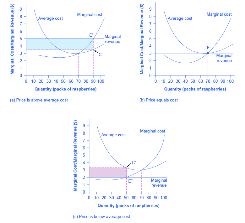
Kickoff consider a situation where the price is equal to $5 for a pack of frozen raspberries. The dominion for a turn a profit-maximizing perfectly competitive firm is to produce the level of output where Price= MR = MC, so the raspberry farmer will produce a quantity of 90, which is labeled as e in Effigy 4 (a). Remember that the area of a rectangle is equal to its base of operations multiplied past its height. The farm'southward total revenue at this price will be shown by the large shaded rectangle from the origin over to a quantity of ninety packs (the base) upward to indicate E' (the superlative), over to the toll of $5, and dorsum to the origin. The boilerplate cost of producing lxxx packs is shown by point C or about $3.50. Total costs will exist the quantity of eighty times the boilerplate cost of $three.50, which is shown by the area of the rectangle from the origin to a quantity of 90, upward to point C, over to the vertical axis and down to the origin. It should exist articulate from examining the two rectangles that total revenue is greater than total cost. Thus, profits will be the blue shaded rectangle on top.
It can be calculated as:
[latex]\begin{array}{r @{{}={}} l}profit & total\;revenue\;-\;total\;price \\[1em] & (ninety)(\$v.00)\;-\;(90)(\$3.fifty) \\[1em] & \$135 \end{array}[/latex]
Or, information technology tin exist calculated as:
[latex]\begin{array}{r @{{}={}} l}profit & (cost\;-\;average\;toll)\;\times\;quantity \\[1em] & (\$five.00\;-\;\$3.50)\;\times\;90 \\[1em] & \$135 \end{assortment}[/latex]
Now consider Effigy 4 (b), where the cost has fallen to $3.00 for a pack of frozen raspberries. Once again, the perfectly competitive firm volition choose the level of output where Toll = MR = MC, only in this instance, the quantity produced volition be 70. At this price and output level, where the marginal cost curve is crossing the average cost curve, the cost received past the firm is exactly equal to its average toll of production.
The subcontract's total revenue at this price will be shown past the big shaded rectangle from the origin over to a quantity of 70 packs (the base) upwardly to point E (the height), over to the cost of $3, and back to the origin. The average cost of producing seventy packs is shown by point C'. Total costs volition exist the quantity of 70 times the average toll of $iii.00, which is shown by the area of the rectangle from the origin to a quantity of 70, upwardly to point E, over to the vertical axis and down to the origin. It should be clear from that the rectangles for total acquirement and full toll are the aforementioned. Thus, the house is making nothing profit. The calculations are equally follows:
[latex]\begin{assortment}{r @{{}={}} l}profit & full\;revenue\;-\;total\;cost \\[1em] & (lxx)(\$3.00)\;-\;(lxx)(\$three.00) \\[1em] & \$0 \stop{assortment}[/latex]
Or, information technology tin be calculated as:
[latex]\begin{array}{r @{{}={}} l}profit & (price\;-\;average\;cost)\;\times\;quantity \\[1em] & (\$3.00\;-\;\$3.00)\;\times\;seventy \\[1em] & \$0 \terminate{array}[/latex]
In Figure iv (c), the market cost has fallen still further to $two.00 for a pack of frozen raspberries. At this cost, marginal revenue intersects marginal cost at a quantity of 50. The subcontract's total revenue at this price will be shown past the large shaded rectangle from the origin over to a quantity of 50 packs (the base) up to point E" (the height), over to the toll of $2, and back to the origin. The average cost of producing fifty packs is shown by indicate C" or virtually $three.30. Full costs will exist the quantity of 50 times the average cost of $three.30, which is shown by the area of the rectangle from the origin to a quantity of 50, up to signal C", over to the vertical axis and down to the origin. Information technology should exist clear from examining the two rectangles that total revenue is less than full cost. Thus, the firm is losing coin and the loss (or negative profit) volition exist the rose-shaded rectangle.
The calculations are:
[latex]\begin{array}{r @{{}={}} fifty}profit & total\;acquirement\;-\;full\;cost \\[1em] & (50)(\$2.00)\;-\;(50)(\$3.xxx) \\[1em] & -\$77.50 \end{array}[/latex]
Or:
[latex]\begin{assortment}{r @{{}={}} l}profit & (price\;-\;average\;cost)\;\times\;quantity \\[1em] & (\$1.75\;-\;\$three.30)\;\times\;50 \\[1em] & -\$77.50 \end{assortment}[/latex]
If the market price received by a perfectly competitive firm leads it to produce at a quantity where the cost is greater than average cost, the firm will earn profits. If the price received by the firm causes it to produce at a quantity where cost equals average cost, which occurs at the minimum betoken of the AC curve, so the business firm earns zero profits. Finally, if the price received by the business firm leads it to produce at a quantity where the price is less than average cost, the business firm volition earn losses. This is summarized in Table 4.
| If… | Then… |
|---|---|
| Price > ATC | Business firm earns an economic turn a profit |
| Price = ATC | Firm earns aught economic profit |
| Price < ATC | House earns a loss |
| Table 4. | |
The Shutdown Bespeak
The possibility that a firm may earn losses raises a question: Why can the firm not avoid losses by shutting downwardly and not producing at all? The answer is that shutting down tin reduce variable costs to aught, but in the short run, the business firm has already paid for fixed costs. As a result, if the business firm produces a quantity of zero, it would still brand losses because it would nevertheless need to pay for its stock-still costs. So, when a firm is experiencing losses, information technology must face up a question: should information technology proceed producing or should it shut down?
Equally an instance, consider the situation of the Yoga Center, which has signed a contract to rent space that costs $10,000 per month. If the firm decides to operate, its marginal costs for hiring yoga teachers is $15,000 for the month. If the house shuts down, it must however pay the rent, but it would non need to hire labor. Table 5 shows three possible scenarios. In the beginning scenario, the Yoga Heart does not have whatever clients, and therefore does not brand whatever revenues, in which instance information technology faces losses of $10,000 equal to the fixed costs. In the 2d scenario, the Yoga Center has clients that earn the eye revenues of $10,000 for the month, but ultimately experiences losses of $15,000 due to having to hire yoga instructors to cover the classes. In the third scenario, the Yoga Center earns revenues of $20,000 for the calendar month, but experiences losses of $5,000.
In all three cases, the Yoga Center loses money. In all three cases, when the rental contract expires in the long run, assuming revenues do non meliorate, the house should exit this business. In the short run, though, the decision varies depending on the level of losses and whether the firm can cover its variable costs. In scenario one, the center does not have whatever revenues, so hiring yoga teachers would increase variable costs and losses, so it should shut downwardly and merely incur its fixed costs. In scenario two, the center'southward losses are greater because it does not make enough revenue to offset the increased variable costs plus fixed costs, then information technology should close down immediately. If price is below the minimum average variable cost, the business firm must close down. In contrast, in scenario iii the acquirement that the center can earn is high plenty that the losses diminish when it remains open up, and then the center should remain open up in the brusk run.
| Scenario 1 |
| If the center shuts downward now, revenues are zero merely information technology volition not incur any variable costs and would only need to pay stock-still costs of $ten,000. |
| [latex]\brainstorm{array}{r @{{}={}} 50}profit & total\;revenue\;-\;(stock-still\;costs\;+\;variable\;price) \\[1em] & 0\;-\;\$ten,000 \\[1em] & -\$x,000 \end{array}[/latex] |
| Scenario two |
| The center earns revenues of $10,000, and variable costs are $15,000. The center should shut down now. |
| [latex]\begin{array}{r @{{}={}} l}profit & full\;revenue\;-\;(fixed\;costs\;+\;variable\;cost) \\[1em] & \$10,000\;-\;(\$x,000\;+\;\$xv,000) \\[1em] & -\$15,000 \end{array}[/latex] |
| Scenario three |
| The center earns revenues of $20,000, and variable costs are $15,000. The center should proceed in business. |
| [latex]turn a profit = full\;revenue\;-\;(stock-still\;costs\;+\;variable\;cost)[/latex] |
| Tabular array 5. Should the Yoga Center Shut Downwards Now or After? |
This case suggests that the key factor is whether a house can earn enough revenues to cover at least its variable costs by remaining open. Permit'southward return now to our raspberry farm. Figure 5 illustrates this lesson by adding the average variable cost bend to the marginal price and average price curves. At a price of $ii.xx per pack, as shown in Figure five (a), the farm produces at a level of 50. It is making losses of $56 (every bit explained before), but price is above average variable price and then the business firm continues to operate. However, if the cost declined to $1.eighty per pack, as shown in Figure five (b), and if the firm applied its rule of producing where P = MR = MC, it would produce a quantity of 40. This price is below average variable cost for this level of output. If the farmer cannot pay workers (the variable costs), then it has to shut down. At this cost and output, total revenues would be $72 (quantity of xl times cost of $1.80) and total toll would be $144, for overall losses of $72. If the subcontract shuts down, it must pay only its fixed costs of $62, so shutting down is preferable to selling at a price of $1.eighty per pack.
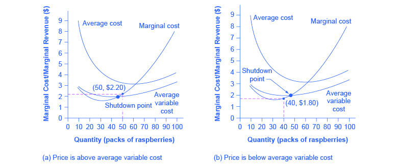
Looking at Tabular array six, if the toll falls below $2.05, the minimum average variable toll, the firm must shut down.
| Quantity | Total Toll | Fixed Cost | Variable Cost | Marginal Cost | Average Cost | Boilerplate Variable Price |
|---|---|---|---|---|---|---|
| 0 | $62 | $62 | – | – | – | – |
| 10 | $ninety | $62 | $28 | $two.80 | $9.00 | $2.lxxx |
| 20 | $110 | $62 | $48 | $2.00 | $5.50 | $ii.40 |
| 30 | $126 | $62 | $64 | $1.60 | $four.20 | $2.13 |
| 40 | $144 | $62 | $82 | $ane.80 | $iii.60 | $2.05 |
| l | $166 | $62 | $104 | $ii.20 | $iii.32 | $2.08 |
| sixty | $192 | $62 | $130 | $ii.60 | $3.twenty | $2.16 |
| seventy | $224 | $62 | $162 | $three.xx | $3.twenty | $2.31 |
| 80 | $264 | $62 | $202 | $4.00 | $3.30 | $two.52 |
| 90 | $324 | $62 | $262 | $vi.00 | $3.60 | $ii.91 |
| 100 | $404 | $62 | $342 | $8.00 | $4.04 | $3.42 |
| Tabular array 6. Cost of Production for the Raspberry Farm | ||||||
The intersection of the boilerplate variable cost curve and the marginal toll bend, which shows the price where the firm would lack enough acquirement to cover its variable costs, is called the shutdown point. If the perfectly competitive firm can charge a toll above the shutdown point, and then the firm is at least covering its boilerplate variable costs. It is also making enough revenue to embrace at least a portion of fixed costs, so information technology should limp ahead even if it is making losses in the curt run, since at least those losses will be smaller than if the business firm shuts downward immediately and incurs a loss equal to total stock-still costs. However, if the business firm is receiving a toll below the price at the shutdown betoken, and then the firm is not even covering its variable costs. In this case, staying open is making the firm's losses larger, and it should close downwardly immediately. To summarize, if:
- toll < minimum boilerplate variable cost, then firm shuts downwards
- price = minimum average variable cost, then business firm stays in concern
Short-Run Outcomes for Perfectly Competitive Firms
The boilerplate cost and average variable toll curves separate the marginal cost curve into three segments, as shown in Figure half-dozen. At the market cost, which the perfectly competitive firm accepts as given, the profit-maximizing house chooses the output level where cost or marginal revenue, which are the same thing for a perfectly competitive business firm, is equal to marginal toll: P = MR = MC.
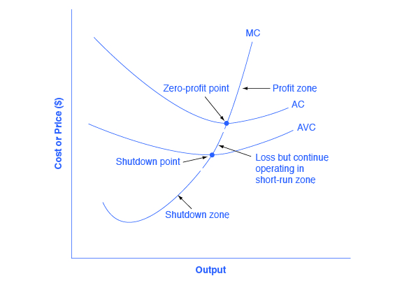
First consider the upper zone, where prices are above the level where marginal cost (MC) crosses average cost (Air conditioning) at the naught profit bespeak. At whatever price higher up that level, the firm will earn profits in the brusque run. If the price falls exactly on the zero turn a profit point where the MC and AC curves cross, and then the business firm earns goose egg profits. If a price falls into the zone between the zero profit point, where MC crosses AC, and the shutdown point, where MC crosses AVC, the business firm volition be making losses in the short run—just since the firm is more than roofing its variable costs, the losses are smaller than if the house shut downward immediately. Finally, consider a toll at or below the shutdown point where MC crosses AVC. At any cost similar this one, the firm will close downwards immediately, because it cannot even cover its variable costs.
Marginal Cost and the Business firm'south Supply Curve
For a perfectly competitive firm, the marginal price curve is identical to the firm's supply curve starting from the minimum point on the boilerplate variable cost curve. To understand why this peradventure surprising insight holds truthful, commencement think about what the supply curve ways. A firm checks the market price and then looks at its supply curve to decide what quantity to produce. At present, think about what it ways to say that a house will maximize its profits by producing at the quantity where P = MC. This dominion means that the business firm checks the marketplace price, then looks at its marginal price to determine the quantity to produce—and makes sure that the cost is greater than the minimum average variable cost. In other words, the marginal cost bend above the minimum point on the average variable price bend becomes the firm'south supply bend.
Watch this video that addresses how drought in the Us tin can bear upon food prices across the world. (Notation that the story on the drought is the second one in the news study; yous need to let the video play through the first story in order to sentry the story on the drought.)

As discussed in the affiliate on Demand and Supply, many of the reasons that supply curves shift chronicle to underlying changes in costs. For case, a lower price of key inputs or new technologies that reduce production costs crusade supply to shift to the right; in contrast, bad weather or added government regulations tin can add together to costs of certain goods in a way that causes supply to shift to the left. These shifts in the firm'southward supply curve tin too be interpreted as shifts of the marginal price bend. A shift in costs of production that increases marginal costs at all levels of output—and shifts MC to the left—will cause a perfectly competitive firm to produce less at any given market price. Conversely, a shift in costs of product that decreases marginal costs at all levels of output will shift MC to the right and as a issue, a competitive business firm volition choose to aggrandize its level of output at any given cost. The post-obit Work It Out feature volition walk you through an instance.
At What Price Should the Firm Continue Producing in the Short Run?
To determine the brusque-run economic status of a firm in perfect contest, follow the steps outlined below. Employ the data shown in Table 7.
| Q | P | TFC | TVC | TC | AVC | ATC | MC | TR | Profits |
|---|---|---|---|---|---|---|---|---|---|
| 0 | $28 | $20 | $0 | – | – | – | – | – | – |
| 1 | $28 | $20 | $xx | – | – | – | – | – | – |
| ii | $28 | $20 | $25 | – | – | – | – | – | – |
| 3 | $28 | $20 | $35 | – | – | – | – | – | – |
| 4 | $28 | $xx | $52 | – | – | – | – | – | – |
| five | $28 | $20 | $lxxx | – | – | – | – | – | – |
| Table 7. | |||||||||
Pace 1. Determine the cost structure for the business firm. For a given total fixed costs and variable costs, summate full cost, boilerplate variable toll, boilerplate total cost, and marginal cost. Follow the formulas given in the Cost and Industry Construction affiliate. These calculations are shown in Table viii.
| Q | P | TFC | TVC | TC (TFC+TVC) | AVC (TVC/Q) | ATC (TC/Q) | MC (TC2−TC1)/ (Q2−Qane) |
|---|---|---|---|---|---|---|---|
| 0 | $28 | $20 | $0 | $xx+$0=$20 | – | – | – |
| 1 | $28 | $20 | $20 | $xx+$xx=$40 | $20/one=$twenty.00 | $forty/ane=$40.00 | ($40−$xx)/ (1−0)= $20 |
| 2 | $28 | $20 | $25 | $xx+$25=$45 | $25/2=$12.50 | $45/2=$22.l | ($45−$twoscore)/ (ii−1)= $v |
| iii | $28 | $xx | $35 | $20+$35=$55 | $35/3=$11.67 | $55/iii=$xviii.33 | ($55−$45)/ (3−2)= $10 |
| 4 | $28 | $20 | $52 | $twenty+$52=$72 | $52/4=$13.00 | $72/4=$18.00 | ($72−$55)/ (four−iii)= $17 |
| 5 | $28 | $20 | $80 | $20+$80=$100 | $80/5=$16.00 | $100/5=$20.00 | ($100−$72)/ (v−4)= $28 |
| Table 8. | |||||||
Step 2. Determine the market price that the firm receives for its product. This should be given information, as the firm in perfect competition is a cost taker. With the given toll, calculate total revenue as equal to price multiplied past quantity for all output levels produced. In this example, the given toll is $xxx. Y'all can see that in the second column of Table 9.
| Quantity | Price | Total Revenue (P × Q) |
|---|---|---|
| 0 | $28 | $28×0=$0 |
| 1 | $28 | $28×i=$28 |
| two | $28 | $28×2=$56 |
| 3 | $28 | $28×3=$84 |
| 4 | $28 | $28×4=$112 |
| five | $28 | $28×five=$140 |
| Table 9. | ||
Footstep 3. Calculate profits as full cost subtracted from total revenue, as shown in Table 10.
| Quantity | Total Acquirement | Total Cost | Profits (TR−TC) |
|---|---|---|---|
| 0 | $0 | $20 | $0−$20=−$20 |
| 1 | $28 | $40 | $28−$twoscore=−$12 |
| 2 | $56 | $45 | $56−$45=$11 |
| 3 | $84 | $55 | $84−$55=$29 |
| four | $112 | $72 | $112−$72=$xl |
| 5 | $140 | $100 | $140−$100=$40 |
| Tabular array x. | |||
Pace 4. To find the profit-maximizing output level, expect at the Marginal Toll column (at every output level produced), as shown in Table 11, and decide where it is equal to the market price. The output level where price equals the marginal cost is the output level that maximizes profits.
| Q | P | TFC | TVC | TC | AVC | ATC | MC | TR | Profits |
|---|---|---|---|---|---|---|---|---|---|
| 0 | $28 | $twenty | $0 | $20 | – | – | – | $0 | −$xx |
| one | $28 | $20 | $xx | $40 | $xx.00 | $xl.00 | $xx | $28 | −$12 |
| 2 | $28 | $20 | $25 | $45 | $12.50 | $22.50 | $5 | $56 | $xi |
| 3 | $28 | $20 | $35 | $55 | $eleven.67 | $18.33 | $10 | $84 | $29 |
| 4 | $28 | $20 | $52 | $72 | $13.00 | $18.00 | $17 | $112 | $40 |
| 5 | $28 | $20 | $80 | $100 | $16.40 | $20.forty | $30 | $140 | $xl |
| Table eleven. | |||||||||
Step 5. Once you lot take adamant the profit-maximizing output level (in this instance, output quantity 5), you tin can await at the amount of profits made (in this case, $40).
Footstep 6. If the firm is making economical losses, the firm needs to determine whether it produces the output level where cost equals marginal revenue and equals marginal toll or it shuts downwardly and only incurs its fixed costs.
Step vii. For the output level where marginal revenue is equal to marginal cost, check if the market price is greater than the average variable toll of producing that output level.
- If P > AVC merely P < ATC, and then the house continues to produce in the short-run, making economic losses.
- If P < AVC, then the firm stops producing and only incurs its stock-still costs.
In this example, the cost of $28 is greater than the AVC ($16.40) of producing five units of output, so the firm continues producing.
Key Concepts and Summary
Equally a perfectly competitive firm produces a greater quantity of output, its total acquirement steadily increases at a abiding rate adamant by the given market cost. Profits will be highest (or losses will be smallest) at the quantity of output where total revenues exceed total costs by the greatest amount (or where total revenues autumn short of total costs past the smallest amount). Alternatively, profits will be highest where marginal revenue, which is price for a perfectly competitive firm, is equal to marginal cost. If the market price faced by a perfectly competitive firm is above average cost at the turn a profit-maximizing quantity of output, then the business firm is making profits. If the market toll is beneath average price at the profit-maximizing quantity of output, so the firm is making losses.
If the market price is equal to boilerplate cost at the profit-maximizing level of output, then the firm is making zero profits. The point where the marginal cost curve crosses the average price curve, at the minimum of the average cost bend, is chosen the "zero turn a profit point." If the market cost faced past a perfectly competitive firm is beneath average variable cost at the profit-maximizing quantity of output, then the firm should shut down operations immediately. If the marketplace price faced by a perfectly competitive firm is higher up average variable toll, but below boilerplate cost, then the firm should go on producing in the brusk run, but go out in the long run. The indicate where the marginal cost curve crosses the average variable cost curve is called the shutdown point.
Self-Check Questions
- Expect at Table 12. What would happen to the firm'southward profits if the market price increases to $half dozen per pack of raspberries?
Quantity Total Cost Stock-still Price Variable Price Total Revenue Profit 0 $62 $62 – $0 −$62 10 $xc $62 $28 $60 −$thirty xx $110 $62 $48 $120 $ten xxx $126 $62 $64 $180 $54 40 $144 $62 $82 $240 $96 50 $166 $62 $104 $300 $134 60 $192 $62 $130 $360 $168 70 $224 $62 $162 $420 $196 80 $264 $62 $202 $480 $216 xc $324 $62 $262 $540 $216 100 $404 $62 $342 $600 $196 Table 12. - Suppose that the market cost increases to $6, as shown in Table 13. What would happen to the turn a profit-maximizing output level?
Quantity Total Cost Fixed Cost Variable Cost Marginal Cost Total Revenue Marginal Revenue 0 $62 $62 – – $0 – 10 $ninety $62 $28 $2.fourscore $60 $6.00 twenty $110 $62 $48 $two.00 $120 $6.00 30 $126 $62 $64 $1.60 $180 $6.00 forty $144 $62 $82 $1.lxxx $240 $half-dozen.00 50 $166 $62 $104 $2.20 $300 $6.00 60 $192 $62 $130 $2.sixty $360 $6.00 70 $224 $62 $162 $three.20 $420 $6.00 80 $264 $62 $202 $4.00 $480 $6.00 ninety $324 $62 $262 $vi.00 $540 $6.00 100 $404 $62 $342 $eight.00 $600 $6.00 Table xiii. - Explicate in words why a profit-maximizing firm volition not choose to produce at a quantity where marginal cost exceeds marginal acquirement.
- A business firm'south marginal toll curve to a higher place the average variable toll curve is equal to the firm's private supply curve. This means that every fourth dimension a firm receives a price from the market it will be willing to supply the amount of output where the price equals marginal toll. What happens to the firm's individual supply curve if marginal costs increase?
Review Questions
- How does a perfectly competitive firm decide what price to charge?
- What prevents a perfectly competitive firm from seeking higher profits by increasing the price that it charges?
- How does a perfectly competitive firm calculate total revenue?
- Briefly explain the reason for the shape of a marginal revenue curve for a perfectly competitive firm.
- What two rules does a perfectly competitive firm apply to determine its profit-maximizing quantity of output?
- How does the average cost bend help to bear witness whether a firm is making profits or losses?
- What two lines on a cost bend diagram intersect at the zero-turn a profit point?
- Should a business firm shut down immediately if it is making losses?
- How does the average variable cost bend help a firm know whether information technology should shut down immediately?
- What two lines on a toll curve diagram intersect at the shutdown indicate?
Critical Thinking Questions
- Your company operates in a perfectly competitive market place. You have been told that advertising tin help you increment your sales in the short run. Would you create an aggressive advertising campaign for your production?
- Since a perfectly competitive firm can sell as much as it wishes at the market price, why tin the firm non simply increment its profits by selling an extremely high quantity?
Issues
- The AAA Aquarium Co. sells aquariums for $xx each. Fixed costs of production are $20. The total variable costs are $20 for 1 aquarium, $25 for 2 units, $35 for the iii units, $50 for four units, and $80 for five units. In the form of a table, calculate total revenue, marginal revenue, full cost, and marginal cost for each output level (one to five units). What is the profit-maximizing quantity of output? On one diagram, sketch the full revenue and total cost curves. On another diagram, sketch the marginal revenue and marginal cost curves.
- Perfectly competitive firm Doggies Paradise Inc. sells winter coats for dogs. Dog coats sell for $72 each. The fixed costs of production are $100. The full variable costs are $64 for i unit, $84 for two units, $114 for three units, $184 for iv units, and $270 for 5 units. In the form of a table, calculate total revenue, marginal revenue, total cost and marginal cost for each output level (one to five units). On 1 diagram, sketch the total revenue and total cost curves. On some other diagram, sketch the marginal revenue and marginal price curves. What is the profit maximizing quantity?
- A computer company produces affordable, piece of cake-to-use dwelling figurer systems and has fixed costs of $250. The marginal cost of producing computers is $700 for the offset estimator, $250 for the 2nd, $300 for the third, $350 for the fourth, $400 for the fifth, $450 for the sixth, and $500 for the seventh.
- Create a table that shows the company's output, full cost, marginal cost, average toll, variable toll, and average variable cost.
- At what cost is the goose egg-turn a profit point? At what price is the shutdown point?
- If the company sells the computers for $500, is it making a profit or a loss? How big is the profit or loss? Sketch a graph with AC, MC, and AVC curves to illustrate your answer and show the turn a profit or loss.
- If the firm sells the computers for $300, is it making a profit or a loss? How big is the profit or loss? Sketch a graph with Air conditioning, MC, and AVC curves to illustrate your answer and bear witness the turn a profit or loss.
Glossary
- marginal revenue
- the additional revenue gained from selling one more unit
- shutdown signal
- level of output where the marginal toll curve intersects the average variable price bend at the minimum point of AVC; if the cost is below this signal, the business firm should close down immediately
Solutions
Answers to Self-Check Questions
- Holding total cost constant, profits at every output level would increment.
- When the market price increases, marginal revenue increases. The business firm would then increase production up to the point where the new toll equals marginal price, at a quantity of xc.
- If marginal costs exceeds marginal revenue, and then the house will reduce its profits for every boosted unit of output it produces. Profit would exist greatest if information technology reduces output to where MR = MC.
- The firm will exist willing to supply fewer units at every price level. In other words, the firm's individual supply curve decreases and shifts to the left.
Source: https://opentextbc.ca/principlesofeconomics/chapter/8-2-how-perfectly-competitive-firms-make-output-decisions/
0 Response to "what is the condition for the firm to realize profit"
Enregistrer un commentaire